Option Pricing With Neural Networks
Introduction
In this post I will shed some light on recent advances in machine learning applied to financial markets. Specifically focusing on the use of neural networks for pricing and hedging of derivative securities.
Background
Derivatives are financial instruments that derive their value from an underlying asset such as a commodity, equity, currency, or bond. Derivatives are primarily used by investors for speculation and hedging. Due to their often complex nature, derivatives can also be used in arbitrage strategies.
Futures
An example of a derivative is a Futures contract, which gives the owner the right to purchase an asset such as a commodity at a pre-specified price, some time in the future. As an example of a scenario where an investor may wish to use a futures contract, consider a soy bean farmer. This farmer has an excess yield of soy-beans in the summer and wishes to stockpile a subset of the soy-bean yield to sell in the middle of the winter when there is likely to be less supply. The farmer wishes to do this, so that they can get a better price for the crops and also to spread their revenue across a longer time period. What the farmer does not know, is what the market price for a bushel of soy-beans in the winter (when he/she wishes to sell). What the farmer may wish to do is the hedge their exposure to the price of soybeans buy entering into a Future’s contract. The farmer will agree to sell his/her Soybeans at a pre agreed upon price at a pre-specified time in the future (Maturity). For this example let’s say the farmer will sell 10 bushels of soy-beans at a price of $100 per bushel, 6 months from now, during the winter. In this example the $100 is called the forward price. As is the case for most contracts, there must be a counter-party that agrees to buy the soybeans at the maturity date for the forward price. In this particular example, the farmer is short soybeans contracts by protecting himself/herself against the price of soybeans going down, and the counter-party that agrees to be on the other side of this contract is long soybeans and expects the price to be greater than $100 by the time the contract expires.
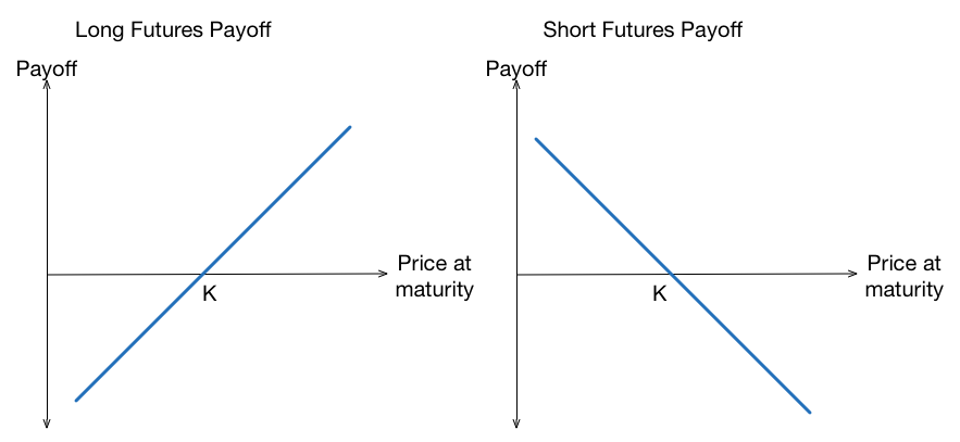
A futures contract payoff function is linear. This means that as the spot value of the underlying asset changes, the contract value changes linearly. Another way of saying this is that the derivative (mathematical) of the value of a futures contract with respect to the underlying asset is 1. We define this derivative as \(\Delta = \frac{\partial V}{\partial S}\), linear payoffs are also sometimes called Delta-One instruments for this reason. The payoff function of a futures contract is outlined in equation \eqref{eq:FutPayoff}.
\begin{equation} P_{EuropeanCallOption} =I * (S-K) \label{eq:FutPayoff} \end{equation}
Where \(I\) is an indicator function that is \(1\) if we are long a Futures contract and \(-1\) if we are short. \(S\) is the spot price of the underlying asset, and \(K\) is the pre agreed upon sale price.
We can display the payoff of a Futures contract graphically by plotting the payoff as a function of strike price for at a given maturity.
Options
Options are a derivative instrument that add an additional sprinkle of complexity (convexity) on top of a contract which has a linear payoff such as a Futures contract or a swap. Options, as their name suggest give the owner, the option to exercise the contract. There are different flavours of optionality that can be applied to a derivative instrument. These flavours often define at what point the owner of the contract can exercise said optionality. Some examples of different styles of options are outlined below.
- European Style Option
- American Style Option
- Bermudan Style Option
- Asian Option
- Barrier Option
European Options
European options are the plain vanilla options that most people would be familiar with. Like a Futures contract, options have a maturity \(T\). Options also add a price sensitive component called the strike price \(K\). For a European The payoff of a European call option is outlined below in \eqref{eq:CallPayoff}
\begin{equation} P_{EuropeanCallOption} = \max(I*(S-K)),0) \label{eq:CallPayoff} \end{equation}
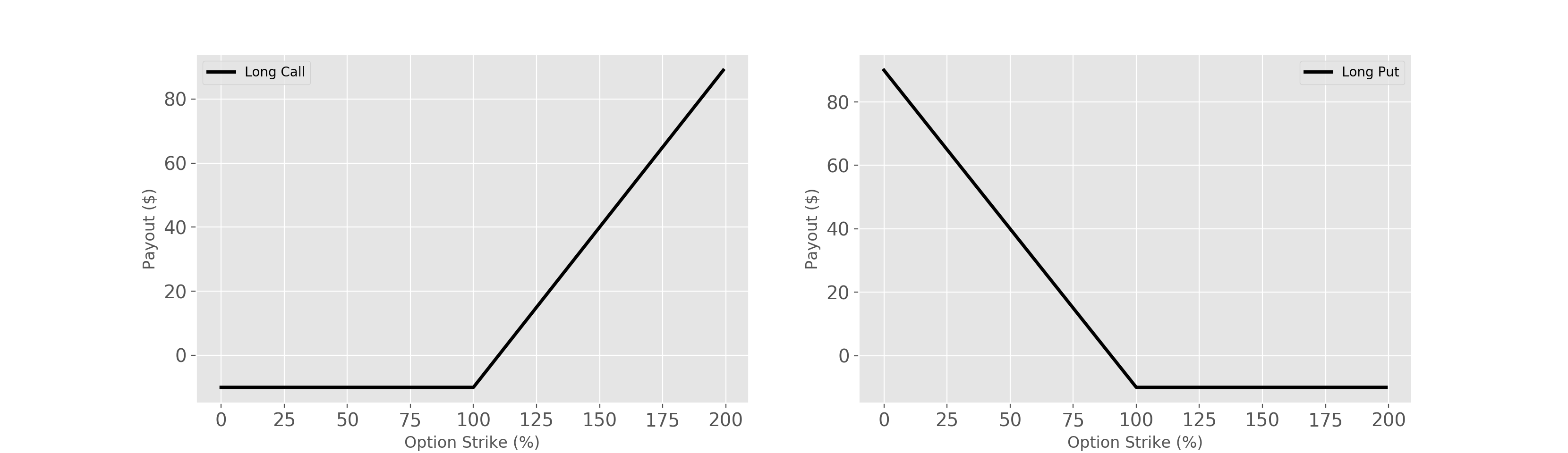
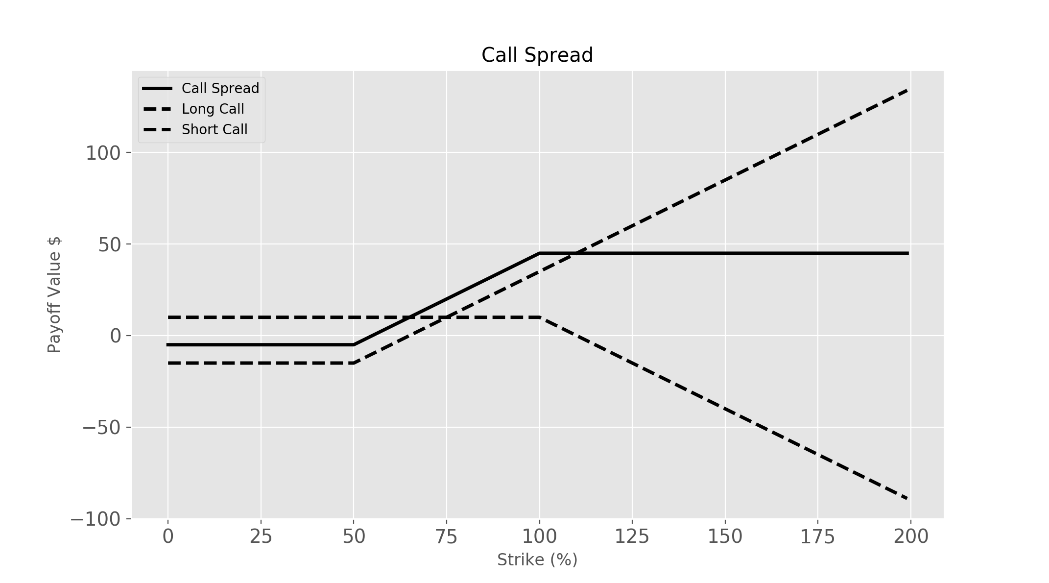
Call and Put Options are the elementary units of derivatives, from these simple options we can construct more complex payoffs that better suit an investment strategy. A simple example of a structure which is made up of a combination of two call options is a call spread. A call spread consist of one long call option and one short call option at different strike prices.
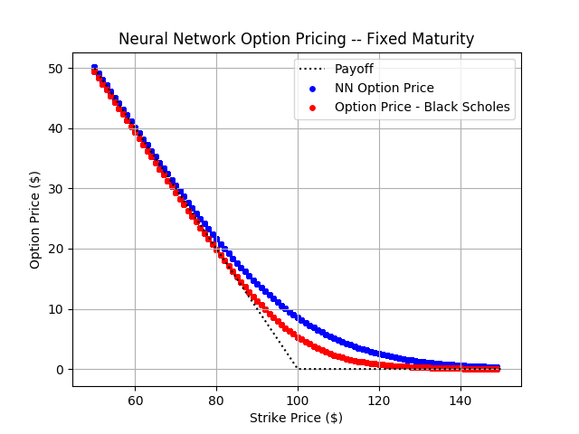
Option Pricing
The traditional method of pricing derivative contracts at a high level is quite simple. We wish to compute the expected value of the contract at some point in the future (maturity) and then discount that value to present day.
Consider an arbitrary derivative payoff functions \(P^* \). The fair value of a derivative contract with payoff \(P^* \) is:
\begin{equation} e^{-r\tau}\mathbb{E}[P^*] \label{eq:FairValue} \end{equation}
Black-Scholes Model
The Black-Scholes model is the most ubiquitous (prototypical) derivative pricing model.
\begin{equation} C(S,k,t,\sigma) = \mathcal{N}(d_1) - ke^{-r \tau}\mathcal{N}(d_2) \label{eq:BlackScholes} \end{equation}
Neural Networks
PyTorch
def print_hi(name)
  puts "Hi, #{name}"
end
print_hi('Tom')
#=> prints 'Hi, Tom' to STDOUT.
Results